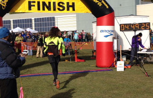
Equinox Marathon finish
It’s the beginning of a new year and time for me to look back at what I learned last year. Rather than a long narrative, let’s focus on the data. The local newspaper did a “community profile” of me this year and it was focused on my curiosity about the world around us and how we can measure and analyze it to better understand our lives. This post is a brief summary of that sort of analysis for my small corner of the world in the year that was 2013.
Exercise
2013 was the year I decided to, and did, run the Equinox Marathon, so I spent a lot of time running this year and a lot less time bicycling. Since the race, I’ve been having hip problems that have kept me from skiing or running much at all. The roads aren’t cleared well enough to bicycle on them in the winter so I got a fat bike to commute on the trails I’d normally ski.
Here are my totals in tabular form:
| type | miles | hours | calories |
|---|---|---|---|
| Running | 529 | 89 | 61,831 |
| Bicycling | 1,018 | 82 | 54,677 |
| Skiing | 475 | 81 | 49,815 |
| Hiking | 90 | 43 | 18,208 |
| TOTAL | 2,113 | 296 | 184,531 |
I spent just about the same amount of time running, bicycling and skiing this year, and much less time hiking around on the trails than in the past. Because of all the running, and my hip injury, I didn’t manage to commute to work with non-motorized transport quite as much this year (55% of work days instead of 63% in 2012), but the exercise totals are all higher.
One new addition this year is a heart rate monitor, which allows me to much more accurately estimate energy consumption than formulas based on the type of activity, speed, and time. Riding my fat bike, it’s pretty clear that this form of travel is so much less efficient than a road bike with smooth tires that it can barely be called “bicycling,” at least in terms of how much energy it takes to travel over a certain distance.
Here’s the equations from Keytel LR, Goedecke JH, Noakes TD, Hiiloskorpi H, Laukkanen R, van der Merwe L, Lambert EV. 2005. Prediction of energy expenditure from heart rate monitoring during submaximal exercise. J Sports Sci. 23(3):289-97.
where
- hr = Heart rate (in beats/minute)
- w = Weight (in pounds)
- a = Age (in years)
- t = Exercise duration time (in hours)
And a SQL function that implements the version for men (to use it, you’d replace
the nnn and yyyy-mm-dd with the appropriate values for you):
--- Kcalories burned based on average heart rate and number
--- of hours at that rate.
CREATE OR REPLACE FUNCTION kcal_from_hr(hr numeric, hours numeric)
RETURNS numeric
LANGUAGE plpgsql
AS $$
DECLARE
    weight_lb numeric := nnn;
    resting_hr numeric := nn;
    birthday date := 'yyyy-mm-dd';
    resting_kcal numeric;
    exercise_kcal numeric;
BEGIN
    resting_kcal := ((-55.0969+(0.6309*(resting_hr))+
                    (0.0901*weight_lb)+
                    (0.2017*(extract(epoch from now()-birthday)/
                    (365.242*24*60*60))))/4.184)*60*hours;
    exercise_kcal := ((-55.0969+(0.6309*(hr))+
                     (0.0901*weight_lb)+
                     (0.2017*(extract(epoch from now()-birthday)/
                     (365.242*24*60*60))))/4.184)*60*hours;
    RETURN exercise_kcal - resting_kcal;
END;
$$;
Here’s a graphical comparison of my exercise data over the past four years:
It was a pretty remarkable year, although the drop in exercise this fall is disappointing.
Another way to visualize the 2013 data is in the form of a heatmap, where each block represents a day on the calendar, and the color is how many calories I burned on that day. During the summer you can see my long runs on the weekends showing up in red. Equinox was on September 21st, the last deep red day of the year.
Weather
2013 was quite remarkable for the number of days where the daily temperature was dramatically different from the 30-year average. The heatmap below shows each day in 2013, and the color indicates how many standard deviations that day’s temperature was from the 30-year average. To put the numbers in perspective, approximately 95.5% of all observations will fall within two standard deviations from the mean, and 99.7% will be within three standard deviations. So the very dark red or dark blue squares on the plot below indicate temperature anomalies that happen less than 1% of the time. Of course, in a full year, you’d expect to see a few of these remarkable differences, but 2013 had a lot of remarkable differences.
2013 saw 45 days where the temperature was more than 2 standard deviations from the mean (19 that were colder than normal and 26 that were warmer), something that should only happen 16 days out of a normal year [ 365.25(1 − 0.9545) ]. There were four days ouside of 3 standard deviations from the mean anomaly. Normally there’d only be a single day [ 365.25(1 − 0.9973) ] with such a remarkably cold or warm temperature.
April and most of May were remarkably cold, resulting in many people skiing long past what is normal in Fairbanks. On May first, Fairbanks still had 17 inches of snow on the ground. Late May, almost all of June and the month of October were abnormally warm, including what may be the warmest week on record in Alaska from June 23rd to the 29th. Although it wasn’t exceptional, you can see the brief cold snap preceding and including the Equinox Marathon on September 21st this year. The result was bitter cold temperatures on race day (my hands and feet didn’t get warm until I was climbing Ester Dome Road an hour into the race), as well as an inch or two of snow on most of the trail sections of the course above 1,000 feet.
Most memorable was the ice and wind storm on November 13th and 14th that dumped several inches of snow and instantly freezing rain, followed by record high winds that knocked power out for 14,000 residents of the area, and then a drop in temperatures to colder than ‒20°F. My office didn’t get power restored for four days.
git
I’m moving more and more of my work into git, which is a distributed revision control system (or put another way, it’s a system that stores stuff and keeps track of all the changes). Because it’s distributed, anything I have on my computer at home can be easily replicated to my computer at work or anywhere else, and any changes that I make to these files on any system, are easy to recover anywhere else. And it’s all backed up on the master repository, and all changes are recorded. If I decide I’ve made a mistake, it’s easy to go back to an earlier version.
Using this sort of system for software code is pretty common, but I’m also using
this for normal text files (the docs repository below), and have
starting moving other things into git such as all my eBooks.
The following figure shows the number of file changes made in three of my
repositories over the course of the year. I don’t know why April was such an
active month for Python, but I clearly did a lot of programming that month. The
large number of file changes during the summer in the docs repository is
because I was keeping my running (and physical therapy) logs in that repository.
Dog Barn
The dog barn was the big summer project. It’s a seven by eleven foot building with large dog boxes inside that we keep warm. When the temperatures are too cold for the dogs to stay outside, we put them into their boxes in the dog barn and turn the heat up to 40°F. I have a real-time visualization of the conditions inside and outside the barn, and because the whole thing is run with a small Linux computer and Arduino board, I’m able to collect a lot of data about how the barn is performing.
One such analysis will be to see how much heat the dogs produce when they are in the barn. To estimate that, we need a baseline of how much heat we’re adding at various temperatures in order to keep it at temperature. I haven’t collected enough cold temperature data to really see what the relationship looks like, but here’s the pattern so far.
The graph shows the relationship between the temperature differential between the outside and inside of the barn plotted against the percentage of time the heater is on in order to maintain that differential, for all 12-hour periods where the dogs weren’t in the barn and there’s less than four missing observations. I’ve also run a linear and quadratic regression in order to predict how much heat will be required at various temperature differentials.
The two r2 values shows how much of the variation in heating is explained by the temperature differential for the linear and the quadratic regressions. I know that this isn’t a linear relationship, but that model still fits the data better than the quadratic model does. It may be that it’s some other form of non-linear relationship that’s not well expressed by a second order polynomial.
Once we can predict how much heat it should take to keep the barn warm at a particular temperature differential, we can see how much less heat we’re using when the dogs are in the barn. One complication is that the dogs produce enough moisture when they are in the barn that we need to ventilate it when they are in there. So in addition to the additive heating from the dogs themselves, there will be increased heat losses because we have to keep it better ventilated.
It’ll be an interesting data set.
Power
Power consumption is a concern now that we’ve set up the dog barn and are keeping it heated with an electric heater. It’s an oil-filled radiator-style heater, and uses around 1,100 Watts when it’s on.
This table shows our overall usage by year for the period we have data.
| year | average watts | total KWH |
|---|---|---|
| 2010 | 551 | 4822 |
| 2011 | 493 | 4318 |
| 2012 | 433 | 3792 |
| 2013 | 418 | 3661 |
Our overall energy use continues to go down, which is a little surprising to me, actually, since we eliminated most of the devices known to use a lot electricity (incandescent light bulbs, halogen floodlights) years ago. Despite that, and bringing the dog barn on line in late November, we used less electricity in 2013 than in the prior three years.
Here’s the pattern by month, and year.
The spike in usage in November is a bit concerning, since it’s the highest overall monthly consumption for the past four years. Hopefully this was primarily due to the heavy use of the heater during the final phases of the dog barn construction. December wasn’t a particularly cold month relative to years past, but it’s good to see that our consumption was actually quite low even with the barn heater being on the entire month.
That wraps it up. Have a happy and productive 2014!
How will I do?
My last blog post compared the time for the men who ran both the 2012 Gold Discovery Run and the Equinox Marathon in order to give me an idea of what sort of Equinox finish time I can expect. Here, I’ll do the same thing for the 2012 Santa Claus Half Marathon.
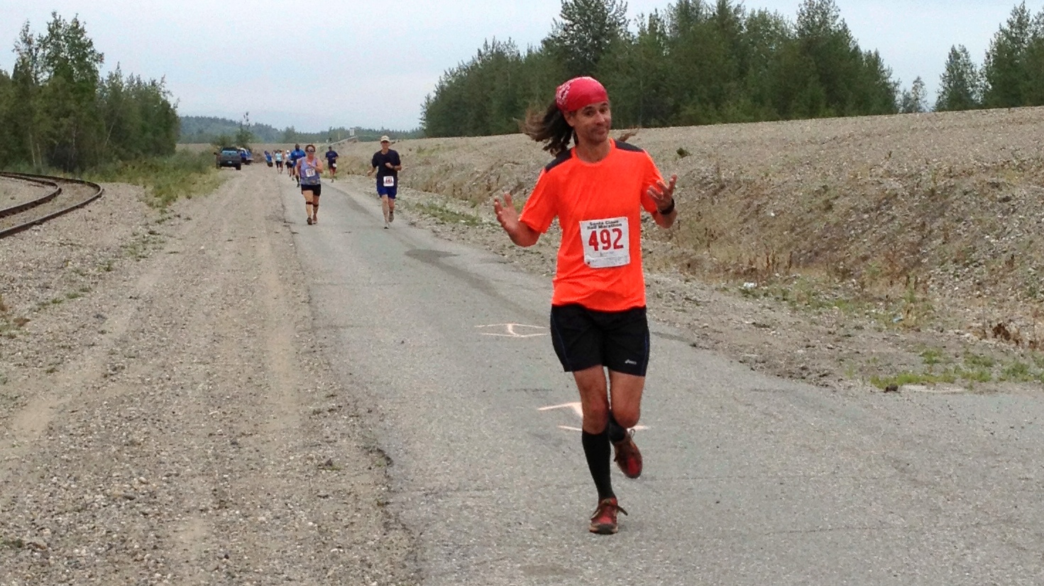
Yesterday I ran the half marathon, finishing in 1:53:08, which is an average pace of 8.63 / 8:38 minutes per mile. I’m recovering from a mild calf strain, so I ran the race very conservatively until I felt like I could trust my legs.
I converted the SportAlaska PDF files the same way as before, and read the data in from the CSV files. Looking at the data, there are a few outliers in this comparison as well. In addition to being ouside of most of the points, they are also times that aren’t close to my expected pace, so are less relevant for predicting my own Equinox finish. Here’s the code to remove them, and perform the linear regression:
combined <- combined[!(combined$sc_pace > 11.0 | combined$eq_pace > 14.5),]
model <- lm(eq_pace ~ sc_pace, data=combined)
summary(model)

Call:
lm(formula = eq_pace ~ sc_pace, data = combined)

Residuals:
     Min       1Q   Median       3Q      Max
-1.08263 -0.39018  0.02476  0.30194  1.27824

Coefficients:
            Estimate Std. Error t value Pr(>|t|)
(Intercept) -1.11209    0.61948  -1.795   0.0793 .
sc_pace      1.44310    0.07174  20.115   <2e-16 ***
---
Signif. codes:  0 ‘***’ 0.001 ‘**’ 0.01 ‘*’ 0.05 ‘.’ 0.1 ‘ ’ 1

Residual standard error: 0.5692 on 45 degrees of freedom
Multiple R-squared: 0.8999,     Adjusted R-squared: 0.8977
F-statistic: 404.6 on 1 and 45 DF,  p-value: < 2.2e-16
There were fewer male runners in 2012 that ran both Santa Claus and Equinox, but we get similar regression statistics. The model and coefficient are significant, and the variation in Santa Claus pace times explains just under 90% of the variation in Equinox times. That’s pretty good.
Here’s a plot of the results:
As before, the blue line shows the model relationship, and the grey area surrounding it shows the 95% confidence interval around that line. This interval represents the range over which 95% of the expected values should appear. The red line is the 1:1 line. As you’d expect for a race twice as long, all the Equinox pace times are significantly slower than for Santa Claus.
There were fewer similar runners in this data set:
| Runner | DOB | Santa Claus | Equinox Time | Equinox Pace |
|---|---|---|---|---|
| John Scherzer | 1972 | 8:17 | 4:49 | 11:01 |
| Greg Newby | 1965 | 8:30 | 5:03 | 11:33 |
| Trent Hubbard | 1972 | 8:31 | 4:48 | 11:00 |
This analysis predicts that I should be able to finish Equinox in just under five hours, which is pretty close to what I found when using Gold Discovery times in my last post. The model predicts a pace of 11:20 and an Equinox finish time of four hours and 57 minutes, and these results are within the range of the three similar runners listed above. Since I was running conservatively in the half marathon, and will probably try to do the same for Equinox, five hours seems like a good goal to shoot for.

Gold Discovery Run, 2013
This spring I ran the Beat Beethoven 5K and had such a good time that I decided to give running another try. I’d tried adding running to my usual exercise routines in the past, but knee problems always sidelined me after a couple months. It’s been three months of slow increases in mileage using a marathon training plan by Hal Higdon, and so far so good.
My goal for this year, beyond staying healthy, is to participate in the 51st running of the Equinox Marathon here in Fairbanks.
One of the challenges for a beginning runner is how pace yourself during a race and how to know what your body can handle. Since Beat Beethoven I've run in the Lulu’s 10K, the Midnight Sun Run (another 10K), and last weekend I ran the 16.5 mile Gold Discovery Run from Cleary Summit down to Silver Gulch Brewery. I completed the race in two hours and twenty-nine minutes, at a pace of 9:02 minutes per mile. Based on this performance, I should be able to estimate my finish time and pace for Equinox by comparing the times for runners that participated in the 2012 Gold Discovery and Equinox.
The first challenge is extracting the data from the PDF files SportAlaska publishes after the race. I found that opening the PDF result files, selecting all the text on each page, and pasting it into a text file is the best way to preserve the formatting of each line. Then I process it through a Python function that extracts the bits I want:
import re
def parse_sportalaska(line):
    """ lines appear to contain:
        place, bib, name, town (sometimes missing), state (sometimes missing),
        birth_year, age_class, class_place, finish_time, off_win, pace,
        points (often missing) """
    fields = line.split()
    place = int(fields.pop(0))
    bib = int(fields.pop(0))
    name = fields.pop(0)
    while True:
        n = fields.pop(0)
        name = '{} {}'.format(name, n)
        if re.search('^[A-Z.-]+$', n):
            break
    pre_birth_year = []
    pre_birth_year.append(fields.pop(0))
    while True:
        try:
            f = fields.pop(0)
        except:
            print("Warning: couldn't parse: '{0}'".format(line.strip()))
            break
        else:
            if re.search('^[0-9]{4}$', f):
                birth_year = int(f)
                break
            else:
                pre_birth_year.append(f)
    if re.search('^[A-Z]{2}$', pre_birth_year[-1]):
        state = pre_birth_year[-1]
        town = ' '.join(pre_birth_year[:-1])
    else:
        state = None
        town = None
    try:
        (age_class, class_place, finish_time, off_win, pace) = fields[:5]
        class_place = int(class_place[1:-1])
        finish_minutes = time_to_min(finish_time)
        fpace = strpace_to_fpace(pace)
    except:
        print("Warning: couldn't parse: '{0}', skipping".format(
              line.strip()))
        return None
    else:
        return (place, bib, name, town, state, birth_year, age_class,
                class_place, finish_time, finish_minutes, off_win,
                pace, fpace)
The function uses a a couple helper functions that convert pace and time strings into floating point numbers, which are easier to analyze.
def strpace_to_fpace(p):
    """ Converts a MM:SS" pace to a float (minutes) """
    (mm, ss) = p.split(':')
    (mm, ss) = [int(x) for x in (mm, ss)]
    fpace = mm + (float(ss) / 60.0)

    return fpace

def time_to_min(t):
    """ Converts an HH:MM:SS time to a float (minutes) """
    (hh, mm, ss) = t.split(':')
    (hh, mm) = [int(x) for x in (hh, mm)]
    ss = float(ss)
    minutes = (hh * 60) + mm + (ss / 60.0)

    return minutes
Once I process the Gold Discovery and Equnox result files through this routine, I dump the results in a properly formatted comma-delimited file, read the data into R and combine the two race results files by matching the runner’s name. Note that these results only include the men competing in the race.
gd <- read.csv('gd_2012_men.csv', header=TRUE)
gd <- gd[,c('name', 'birth_year', 'finish_minutes', 'fpace')]
eq <- read.csv('eq_2012_men.csv', header=TRUE)
eq <- eq[,c('name', 'birth_year', 'finish_minutes', 'fpace')]
combined <- merge(gd, eq, by='name')
names(combined) <- c('name', 'birth_year', 'gd_finish', 'gd_pace',
                     'year', 'eq_finish', 'eq_pace')
When I look at a plot of the data I can see four outliers; two where the runners ran Equinox much faster based on their Gold Discovery pace, and two where the opposite was the case. The two races are two months apart, so I think it’s reasonable to exclude these four rows from the data since all manner of things could happen to a runner in two months of hard training (or on race day!).
attach(combined)
combined <- combined[!((gd_pace > 10 & gd_pace < 11 & eq_pace > 15)
                       | (gd_pace > 15)),]
Let’s test the hypothesis that we can predict Equinox pace from Gold Discovery Pace:
model <- lm(eq_pace ~ birth_year, data=combined)
summary(model)

Call:
lm(formula = eq_pace ~ gd_pace, data = combined)

Residuals:
     Min       1Q   Median       3Q      Max
-1.47121 -0.36833 -0.04207  0.51361  1.42971

Coefficients:
            Estimate Std. Error t value Pr(>|t|)
(Intercept)  0.77392    0.52233   1.482    0.145
gd_pace      1.08880    0.05433  20.042   <2e-16 ***
---
Signif. codes:  0 ‘***’ 0.001 ‘**’ 0.01 ‘*’ 0.05 ‘.’ 0.1 ‘ ’ 1

Residual standard error: 0.6503 on 48 degrees of freedom
Multiple R-squared:  0.8933,    Adjusted R-squared:  0.891
F-statistic: 401.7 on 1 and 48 DF,  p-value: < 2.2e-16
Indeed, we can explain 65% of the variation in Equinox Marathon pace times using Gold Discovery pace times, and both the model and the model coefficient are significant.
Here’s what the results look like:
The red line shows a relationship where the Gold Discovery pace is identical to the Equinox pace for each running. Because the actual data (and the prediced results based on the regression model) are above this line, that means that all the runners were slower in the longer (and harder) Equinox Marathon.
As for me, my 9:02 Gold Discovery pace should translate into an Equinox pace around 10:30. Here are the 2012 runners who were born within ten years of me, and who finished within ten minutes of my 2013 Gold Discovery time:
| Runner | DOB | Gold Discovery | Equinox Time | Equinox Pace |
|---|---|---|---|---|
| Dan Bross | 1964 | 2:24 | 4:20 | 9:55 |
| Chris Hartman | 1969 | 2:25 | 4:45 | 10:53 |
| Mike Hayes | 1972 | 2:27 | 4:58 | 11:22 |
| Ben Roth | 1968 | 2:28 | 4:47 | 10:57 |
| Jim Brader | 1965 | 2:31 | 4:09 | 9:30 |
| Erik Anderson | 1971 | 2:32 | 5:03 | 11:34 |
| John Scherzer | 1972 | 2:33 | 4:49 | 11:01 |
| Trent Hubbard | 1972 | 2:33 | 4:48 | 11:00 |
Based on this, and the regression results, I expect to finish the Equinox Marathon in just under five hours if my training over the next two months goes well.

the swimming hole
Once again, I’ve neglected my blog. My new job, the pressures of getting all our work done this summer, and the rest of life has kept me away.
Events: We’ve taken to swimming in the Creek. During the warmth of early June (which hasn’t returned since…) the Creek temperature rose to 65°F, and swimming was actually quite nice. I’m hoping we’ll get a few more warm days before fall so we can swim out there again.
Projects: I’ve made no progress at all on the new shed, but have repaired the bridge and got our digital antenna installed on the roof. I also replaced our chimney cap with the variety our chimney sweep prefers. Things left to do: Build the shed!, repair the glycol line that keeps the septic pipe thawed, fix and insulate the sewage treatment plant discharge pipe, reinforce the shed roofs, obtain and chop two more cords of firewood, install a heat shield behind the wood stove, get curtains for the two large downstairs windows and the sliding glass doors, and (finally) consider hiring a plumbing and heating company to replace and upgrade our system.
Books: I’ve read quite a few. Here’s a summary judgement on each:
- McSweeney’s Quarterly Concern, Volume 26: Enjoyable fictions, interesting format, no real standouts for me.
- The Rest is Noise: Fantastic look at the music and history of the 20th century. Alex Ross is one of my favorite New Yorker writers and this book doesn’t disappoint.
- Ambitious Brew: Interesting history of beer brewing in the United States. It dispels many of the classic beer myths (the most classic being that the big super-brewers ruined American beer, only to be “saved” by the micros), and tells a great story. Prost!
- Let the Northern Lights Erase Your Name: A very enjoyable book with a very memorable female lead. Vida has a great abbreviated and expressive way of writing that was refreshing.
- The Echo Maker: I’ve been looking forward to this one for so long, that I think the reading of it couldn’t be anything but a disappointment. I enjoyed it as a meditation on brain injury, but I felt like the characters were a little overwrought and stiff.
The rest: Andrea continues to progress toward her goal of running the Equinox Marathon. She’s out running sixteen miles (16 miles!) right now. I’m super proud of her. Meanwhile, I’ve been bicycling to work almost every day (13 miles round-trip) and the two of us are working toward doing 100 push ups in six weeks. Maybe by the next photo of me in the Creek, I’ll be ripped.
Probably not…