Introduction
So far this winter we’ve gotten only 4.1 inches of snow, well below the normal 19.7 inches, and there is only 2 inches of snow on the ground. At this point last year we had 8 inches and I’d been biking and skiing on the trail to work for two weeks. In his North Pacific Temperature Update blog post, Richard James mentions that winters like this one, with a combined strongly positive Pacific Decadal Oscillation phase and strongly negative North Pacific Mode phase tend to be a “distinctly dry” pattern for interior Alaska. I don’t pretend to understand these large scale climate patterns, but I thought it would be interesting to look at snowfall and snow depth in years with very little mid-November snow. In other years like this one do we eventually get enough snow that the trails fill in and we can fully participate in winter sports like skiing, dog mushing, and fat biking?
Data
We will use daily data from the Global Historical Climate Data set for the Fairbanks International Airport station. Data prior to 1950 is excluded because of poor quality snowfall and snow depth data and because there’s a good chance that our climate has changed since then and patterns from that era aren’t a good model for the current climate in Alaska.
We will look at both snow depth and the cumulative winter snowfall.
Results
The following tables show the ten years with the lowest cumulative snowfall and snow depth values from 1950 to the present on November 18th.
| Year | Cumulative Snowfall (inches) |
|---|---|
| 1953 | 1.5 |
| 2016 | 4.1 |
| 1954 | 4.3 |
| 2014 | 6.0 |
| 2006 | 6.4 |
| 1962 | 7.5 |
| 1998 | 7.8 |
| 1960 | 8.5 |
| 1995 | 8.8 |
| 1979 | 10.2 |
| Year | Snow depth (inches) |
|---|---|
| 1953 | 1 |
| 1954 | 1 |
| 1962 | 1 |
| 2016 | 2 |
| 2014 | 2 |
| 1998 | 3 |
| 1964 | 3 |
| 1976 | 3 |
| 1971 | 3 |
| 2006 | 4 |
2016 has the second-lowest cumulative snowfall behind 1953 and is tied for second with 2014 for snow depth with 1953, 1954 and 1962 all having only 1 inch of snow on November 18th.
It also seems like recent years appear in these tables more frequently than would be expected. Grouping by decade and averaging cumulative snowfall and snow depth yields the pattern in the chart below. The error bars (not shown) are fairly large, so the differences between decades aren’t likely to be statistically significant, but there is a pattern of lower snowfall amounts in recent decades.

Now let’s see what happened in those years with low snowfall and snow depth values in mid-November starting with cumulative snowfall. The following plot (and the subsequent snow depth plot) shows the data for the low-value years (and one very high snowfall year—1990), with each year’s data as a separate line. The smooth dark cyan line through the middle of each plot is the smoothed line through the values for all years; a sort of “average” snowfall and snow depth curve.

In all four mid-November low-snowfall years, the cumulative snowfall values remain below average throughout the winter, but snow did continue to fall as the season went on. Even the lowest winter year here, 2006–2007, still ended the winter with 15 inches of snow on the groud.
The following plot shows snow depth for the four years with the lowest snow depth on November 18th. The data is formatted the same as in the previous plot except we’ve jittered the values slightly to make the plot easier to read.

The pattern here is similar, but the snow depths get much closer to the average values. Snow depth for all four low snow years remain low throughout November, but start rising in December, dramatically in 1954 and 2014.
One of the highest snowfall years between 1950 and 2016 was 1990–1991 (shown on both plots). An impressive 32.8 inches of snow fell in eight days between December 21st and December 28th, accounting for the sharp increase in cumulative snowfall and snow depth shown on both plots. There are five years in the record where the cumulative total for the entire winter was lower than these eight days in 1990.
Conclusion
Despite the lack of snow on the ground to this point in the year, the record shows that we are still likely to get enough snow to fill in the trails. We may need to wait until mid to late December, but it’s even possible we’ll eventually reach the long term average depth before spring.
Appendix
Here’s the R code used to generate the statistics, tables and plots from this post:
library(tidyverse)
library(lubridate)
library(scales)
library(knitr)

noaa <- src_postgres(host="localhost", dbname="noaa")

snow <- tbl(noaa, build_sql(
   "WITH wdoy_data AS (
         SELECT dte, dte - interval '120 days' as wdte,
            tmin_c, tmax_c, (tmin_c+tmax_c)/2.0 AS tavg_c,
            prcp_mm, snow_mm, snwd_mm
         FROM ghcnd_pivot
         WHERE station_name = 'FAIRBANKS INTL AP'
         AND dte > '1950-09-01')
   SELECT dte, date_part('year', wdte) AS wyear, date_part('doy', wdte) AS wdoy,
         to_char(dte, 'Mon DD') AS mmdd,
         tmin_c, tmax_c, tavg_c, prcp_mm, snow_mm, snwd_mm
   FROM wdoy_data")) %>%
   mutate(wyear=as.integer(wyear),
            wdoy=as.integer(wdoy),
            snwd_mm=as.integer(snwd_mm)) %>%
   select(dte, wyear, wdoy, mmdd,
            tmin_c, tmax_c, tavg_c, prcp_mm, snow_mm, snwd_mm) %>% collect()

write_csv(snow, "pafa_data_with_wyear_post_1950.csv")
save(snow, file="pafa_data_with_wyear_post_1950.rdata")

cum_snow <- snow %>%
   mutate(snow_na=ifelse(is.na(snow_mm),1,0),
         snow_mm=ifelse(is.na(snow_mm),0,snow_mm)) %>%
   group_by(wyear) %>%
   mutate(snow_mm_cum=cumsum(snow_mm),
         snow_na=cumsum(snow_na)) %>%
   ungroup() %>%
   mutate(snow_in_cum=round(snow_mm_cum/25.4, 1),
         snwd_in=round(snwd_mm/25.4, 0))

nov_18_snow <- cum_snow %>%
   filter(mmdd=='Nov 18') %>%
   select(wyear, snow_in_cum, snwd_in) %>%
   arrange(snow_in_cum)

decadal_avg <- nov_18_snow %>%
   mutate(decade=as.integer(wyear/10)*10) %>%
   group_by(decade) %>%
   summarize(`Snow depth`=mean(snwd_in),
            snwd_sd=sd(snwd_in),
            `Cumulative Snowfall`=mean(snow_in_cum),
            snow_cum_sd=sd(snow_in_cum))

decadal_averages <- ggplot(decadal_avg %>%
                              gather(variable, value, -decade) %>%
                              filter(variable %in% c("Cumulative Snowfall",
                                                      "Snow depth")),
                           aes(x=as.factor(decade), y=value, fill=variable)) +
            theme_bw() +
            geom_bar(stat="identity", position="dodge") +
            scale_x_discrete(name="Decade", breaks=c(1950, 1960, 1970, 1980,
                                                   1990, 2000, 2010)) +
            scale_y_continuous(name="Inches", breaks=pretty_breaks(n=10)) +
            scale_fill_discrete(name="Measurement")

print(decadal_averages)

date_x_scale <- cum_snow %>%
   filter(grepl(' (01|15)', mmdd), wyear=='1994') %>%
   select(wdoy, mmdd)

cumulative_snowfall <-
   ggplot(cum_snow %>% filter(wyear %in% c(1953, 1954, 2014, 2006, 1990),
                              wdoy>183,
                              wdoy<320),
            aes(x=wdoy, y=snow_in_cum, colour=as.factor(wyear))) +
   theme_bw() +
   geom_smooth(data=cum_snow %>% filter(wdoy>183, wdoy<320),
               aes(x=wdoy, y=snow_in_cum),
               size=0.5, colour="darkcyan",
               inherit.aes=FALSE,
               se=FALSE) +
   geom_line(position="jitter") +
   scale_x_continuous(name="",
                     breaks=date_x_scale$wdoy,
                     labels=date_x_scale$mmdd) +
   scale_y_continuous(name="Cumulative snowfall (in)",
                     breaks=pretty_breaks(n=10)) +
   scale_color_discrete(name="Winter year")

print(cumulative_snowfall)

snow_depth <-
   ggplot(cum_snow %>% filter(wyear %in% c(1953, 1954, 1962, 2014, 1990),
                              wdoy>183,
                              wdoy<320),
            aes(x=wdoy, y=snwd_in, colour=as.factor(wyear))) +
   theme_bw() +
   geom_smooth(data=cum_snow %>% filter(wdoy>183, wdoy<320),
               aes(x=wdoy, y=snwd_in),
               size=0.5, colour="darkcyan",
               inherit.aes=FALSE,
               se=FALSE) +
   geom_line(position="jitter") +
   scale_x_continuous(name="",
                     breaks=date_x_scale$wdoy,
                     labels=date_x_scale$mmdd) +
   scale_y_continuous(name="Snow Depth (in)",
                     breaks=pretty_breaks(n=10)) +
   scale_color_discrete(name="Winter year")

print(snow_depth)
Equinox Marathon Relay leg 2, 2016
Introduction
A couple years ago I compared racing data between two races (Gold Discovery and Equinox, Santa Claus and Equinox) in the same season for all runners that ran in both events. The result was an estimate of how fast I might run the Equinox Marathon based on my times for Gold Discovery and the Santa Claus Half Marathon.
Several years have passed and I've run more races and collected more racing data for all the major Fairbanks races and wanted to run the same analysis for all combinations of races.
Data
The data comes from a database I’ve built of race times for all competitors, mostly coming from the results available from Chronotrack, but including some race results from SportAlaska.
We started by loading the required R packages and reading in all the racing data, a small subset of which looks like this.
| race | year | name | finish_time | birth_year | sex |
|---|---|---|---|---|---|
| Beat Beethoven | 2015 | thomas mcclelland | 00:21:49 | 1995 | M |
| Equinox Marathon | 2015 | jennifer paniati | 06:24:14 | 1989 | F |
| Equinox Marathon | 2014 | kris starkey | 06:35:55 | 1972 | F |
| Midnight Sun Run | 2014 | kathy toohey | 01:10:42 | 1960 | F |
| Midnight Sun Run | 2016 | steven rast | 01:59:41 | 1960 | M |
| Equinox Marathon | 2013 | elizabeth smith | 09:18:53 | 1987 | F |
| ... | ... | ... | ... | ... | ... |
Next we loaded in the names and distances of the races and combined this with the individual racing data. The data from Chronotrack doesn’t include the mileage and we will need that to calculate pace (minutes per mile).
My database doesn’t have complete information about all the racers that competed, and in some cases the information for a runner in one race conflicts with the information for the same runner in a different race. In order to resolve this, we generated a list of runners, grouped by their name, and threw out racers where their name matches but their gender was reported differently from one race to the next. Please understand we’re not doing this to exclude those who have changed their gender identity along the way, but to eliminate possible bias from data entry mistakes.
Finally, we combined the racers with the individual racing data, substituting our corrected runner information for what appeared in the individual race’s data. We also calculated minutes per mile (pace) and the age of the runner during the year of the race (age). Because we’re assigning a birth year to the minimum reported year from all races, our age variable won’t change during the running season, which is closer to the way age categories are calculated in Europe. Finally, we removed results where pace was greater than 20 minutes per mile for races longer than ten miles, and greater than 16 minute miles for races less than ten miles. These are likely to be outliers, or competitors not running the race.
| name | birth_year | gender | race_str | year | miles | minutes | pace | age |
|---|---|---|---|---|---|---|---|---|
| aaron austin | 1983 | M | midnight_sun_run | 2014 | 6.2 | 50.60 | 8.16 | 31 |
| aaron bravo | 1999 | M | midnight_sun_run | 2013 | 6.2 | 45.26 | 7.30 | 14 |
| aaron bravo | 1999 | M | midnight_sun_run | 2014 | 6.2 | 40.08 | 6.46 | 15 |
| aaron bravo | 1999 | M | midnight_sun_run | 2015 | 6.2 | 36.65 | 5.91 | 16 |
| aaron bravo | 1999 | M | midnight_sun_run | 2016 | 6.2 | 36.31 | 5.85 | 17 |
| aaron bravo | 1999 | M | spruce_tree_classic | 2014 | 6.0 | 42.17 | 7.03 | 15 |
| ... | ... | ... | ... | ... | ... | ... | ... | ... |
We combined all available results for each runner in all years they participated such that the resulting rows are grouped by runner and year and columns are the races themselves. The values in each cell represent the pace for the runner × year × race combination.
For example, here’s the first six rows for runners that completed Beat Beethoven and the Chena River Run in the years I have data. I also included the column for the Midnight Sun Run in the table, but the actual data has a column for all the major Fairbanks races. You’ll see that two of the six runners listed ran BB and CRR but didn’t run MSR in that year.
| name | gender | age | year | beat_beethoven | chena_river_run | midnight_sun_run |
|---|---|---|---|---|---|---|
| aaron schooley | M | 36 | 2016 | 8.19 | 8.15 | 8.88 |
| abby fett | F | 33 | 2014 | 10.68 | 10.34 | 11.59 |
| abby fett | F | 35 | 2016 | 11.97 | 12.58 | NA |
| abigail haas | F | 11 | 2015 | 9.34 | 8.29 | NA |
| abigail haas | F | 12 | 2016 | 8.48 | 7.90 | 11.40 |
| aimee hughes | F | 43 | 2015 | 11.32 | 9.50 | 10.69 |
| ... | ... | ... | ... | ... | ... | ... |
With this data, we build a whole series of linear models, one for each race combination. We created a series of formula strings and objects for all the combinations, then executed them using map(). We combined the start and predicted race names with the linear models, and used glance() and tidy() from the broom package to turn the models into statistics and coefficients.
All of the models between races were highly significant, but many of them contain coefficients that aren’t significantly different than zero. That means that including that term (age, gender or first race pace) isn’t adding anything useful to the model. We used the significance of each term to reduce our models so they only contained coefficients that were significant and regenerated the statistics and coefficients for these reduced models.
The full R code appears at the bottom of this post.
Results
Here’s the statistics from the ten best performing models (based on R² ).
| start_race | predicted_race | n | R² | p-value |
|---|---|---|---|---|
| run_of_the_valkyries | golden_heart_trail_run | 40 | 0.956 | 0 |
| golden_heart_trail_run | equinox_marathon | 36 | 0.908 | 0 |
| santa_claus_half_marathon | golden_heart_trail_run | 34 | 0.896 | 0 |
| midnight_sun_run | gold_discovery_run | 139 | 0.887 | 0 |
| beat_beethoven | golden_heart_trail_run | 32 | 0.886 | 0 |
| run_of_the_valkyries | gold_discovery_run | 44 | 0.877 | 0 |
| midnight_sun_run | golden_heart_trail_run | 52 | 0.877 | 0 |
| gold_discovery_run | santa_claus_half_marathon | 111 | 0.876 | 0 |
| chena_river_run | golden_heart_trail_run | 44 | 0.873 | 0 |
| run_of_the_valkyries | santa_claus_half_marathon | 91 | 0.851 | 0 |
It’s interesting how many times the Golden Heart Trail Run appears on this list since that run is something of an outlier in the Usibelli running series because it’s the only race entirely on trails. Maybe it’s because it’s distance (5K) is comparable with a lot of the earlier races in the season, but because it’s on trails it matches well with the later races that are at least partially on trails like Gold Discovery or Equinox.
Here are the ten worst models.
| start_race | predicted_race | n | R² | p-value |
|---|---|---|---|---|
| midnight_sun_run | equinox_marathon | 431 | 0.525 | 0 |
| beat_beethoven | hoodoo_half_marathon | 87 | 0.533 | 0 |
| beat_beethoven | midnight_sun_run | 818 | 0.570 | 0 |
| chena_river_run | equinox_marathon | 196 | 0.572 | 0 |
| equinox_marathon | hoodoo_half_marathon | 90 | 0.584 | 0 |
| beat_beethoven | equinox_marathon | 265 | 0.585 | 0 |
| gold_discovery_run | hoodoo_half_marathon | 41 | 0.599 | 0 |
| beat_beethoven | santa_claus_half_marathon | 163 | 0.612 | 0 |
| run_of_the_valkyries | equinox_marathon | 125 | 0.642 | 0 |
| midnight_sun_run | hoodoo_half_marathon | 118 | 0.657 | 0 |
Most of these models are shorter races like Beat Beethoven or the Chena River Run predicting longer races like Equinox or one of the half marathons. Even so, each model explains more than half the variation in the data, which isn’t terrible.
Application
Now that we have all our models and their coefficients, we used these models to make predictions of future performance. I’ve written an online calculator based on the reduced models that let you predict your race results as you go through the running season. The calculator is here: Fairbanks Running Race Converter.
For example, I ran a 7:41 pace for Run of the Valkyries this year. Entering that, plus my age and gender into the converter predicts an 8:57 pace for the first running of the HooDoo Half Marathon. The R² for this model was a respectable 0.71 even though only 23 runners ran both races this year (including me). My actual pace for HooDoo was 8:18, so I came in quite a bit faster than this. No wonder my knee and hip hurt after the race! Using my time from the Golden Heart Trail Run, the converter predicts a HooDoo Half pace of 8:16.2, less than a minute off my 1:48:11 finish.
Appendix: R code
library(tidyverse)
library(lubridate)
library(broom)

races_db <- src_postgres(host="localhost", dbname="races")

combined_races <- tbl(races_db, build_sql(
    "SELECT race, year, lower(name) AS name, finish_time,
        year - age AS birth_year, sex
     FROM chronotrack
     UNION
     SELECT race, year, lower(name) AS name, finish_time,
        birth_year,
        CASE WHEN age_class ~ 'M' THEN 'M' ELSE 'F' END AS sex
     FROM sportalaska
     UNION
     SELECT race, year, lower(name) AS name, finish_time,
        NULL AS birth_year, NULL AS sex
     FROM other"))

races <- tbl(races_db, build_sql(
    "SELECT race,
        lower(regexp_replace(race, '[ ’]', '_', 'g')) AS race_str,
        date_part('year', date) AS year,
        miles
     FROM races"))

racing_data <- combined_races %>%
    inner_join(races) %>%
    filter(!is.na(finish_time))

racers <- racing_data %>%
    group_by(name) %>%
    summarize(races=n(),
              birth_year=min(birth_year),
              gender_filter=ifelse(sum(ifelse(sex=='M',1,0))==
                                   sum(ifelse(sex=='F',1,0)),
                                   FALSE, TRUE),
              gender=ifelse(sum(ifelse(sex=='M',1,0))>
                            sum(ifelse(sex=='F',1,0)),
                            'M', 'F')) %>%
    ungroup() %>%
    filter(gender_filter) %>%
    select(-gender_filter)

racing_data_filled <- racing_data %>%
    inner_join(racers, by="name") %>%
    mutate(birth_year=birth_year.y) %>%
    select(name, birth_year, gender, race_str, year, miles, finish_time) %>%
    group_by(name, race_str, year) %>%
    mutate(n=n()) %>%
    filter(!is.na(birth_year), n==1) %>%
    ungroup() %>%
    collect() %>%
    mutate(fixed=ifelse(grepl('[0-9]+:[0-9]+:[0-9.]+', finish_time),
                        finish_time,
                        paste0('00:', finish_time)),
           minutes=as.numeric(seconds(hms(fixed)))/60.0,
           pace=minutes/miles,
           age=year-birth_year,
           age_class=as.integer(age/10)*10,
           group=paste0(gender, age_class),
           gender=as.factor(gender)) %>%
    filter((miles<10 & pace<16) | (miles>=10 & pace<20)) %>%
    select(-fixed, -finish_time, -n)

speeds_combined <- racing_data_filled %>%
    select(name, gender, age, age_class, group, race_str, year, pace) %>%
    spread(race_str, pace)

main_races <- c('beat_beethoven', 'chena_river_run', 'midnight_sun_run',
                'run_of_the_valkyries', 'gold_discovery_run',
                'santa_claus_half_marathon', 'golden_heart_trail_run',
                'equinox_marathon', 'hoodoo_half_marathon')

race_formula_str <-
    lapply(seq(1, length(main_races)-1),
           function(i)
               lapply(seq(i+1, length(main_races)),
                      function(j) paste(main_races[[j]], '~',
                                        main_races[[i]],
                                        '+ gender', '+ age'))) %>%
    unlist()

race_formulas <- lapply(race_formula_str, function(i) as.formula(i)) %>%
    unlist()

lm_models <- map(race_formulas, ~ lm(.x, data=speeds_combined))

models <- tibble(start_race=factor(gsub('.* ~ ([^ ]+).*',
                                        '\\1',
                                        race_formula_str),
                                   levels=main_races),
                 predicted_race=factor(gsub('([^ ]+).*',
                                            '\\1',
                                            race_formula_str),
                                       levels=main_races),
                 lm_models=lm_models) %>%
    arrange(start_race, predicted_race)

model_stats <- glance(models %>% rowwise(), lm_models)
model_coefficients <- tidy(models %>% rowwise(), lm_models)

reduced_formula_str <- model_coefficients %>%
    ungroup() %>%
    filter(p.value<0.05, term!='(Intercept)') %>%
    mutate(term=gsub('genderM', 'gender', term)) %>%
    group_by(predicted_race, start_race) %>%
    summarize(independent_vars=paste(term, collapse=" + ")) %>%
    ungroup() %>%
    transmute(reduced_formulas=paste(predicted_race, independent_vars, sep=' ~ '))

reduced_formula_str <- reduced_formula_str$reduced_formulas

reduced_race_formulas <- lapply(reduced_formula_str,
                                function(i) as.formula(i)) %>% unlist()

reduced_lm_models <- map(reduced_race_formulas, ~ lm(.x, data=speeds_combined))

n_from_lm <- function(model) {
    summary_object <- summary(model)

    summary_object$df[1] + summary_object$df[2]
}

reduced_models <- tibble(start_race=factor(gsub('.* ~ ([^ ]+).*', '\\1', reduced_formula_str),
                                           levels=main_races),
                         predicted_race=factor(gsub('([^ ]+).*', '\\1', reduced_formula_str),
                                               levels=main_races),
                         lm_models=reduced_lm_models) %>%
    arrange(start_race, predicted_race) %>%
    rowwise() %>%
    mutate(n=n_from_lm(lm_models))

reduced_model_stats <- glance(reduced_models %>% rowwise(), lm_models)
reduced_model_coefficients <- tidy(reduced_models %>% rowwise(), lm_models) %>%
    ungroup()

coefficients_and_stats <- reduced_model_stats %>%
    inner_join(reduced_model_coefficients,
               by=c("start_race", "predicted_race", "n")) %>%
    select(start_race, predicted_race, n, r.squared, term, estimate)

write_csv(coefficients_and_stats,
          "coefficients.csv")

make_scatterplot <- function(start_race, predicted_race) {
   age_limits <- speeds_combined %>%
      filter_(paste("!is.na(", start_race, ")"),
               paste("!is.na(", predicted_race, ")")) %>%
      summarize(min=min(age), max=max(age)) %>%
      unlist()

   q <- ggplot(data=speeds_combined,
               aes_string(x=start_race, y=predicted_race)) +
            # plasma works better with a grey background
            # theme_bw() +
            geom_abline(slope=1, color="darkred", alpha=0.5) +
            geom_smooth(method="lm", se=FALSE) +
            geom_point(aes(shape=gender, color=age)) +
            scale_color_viridis(option="plasma",
                              limits=age_limits) +
            scale_x_continuous(breaks=pretty_breaks(n=10)) +
            scale_y_continuous(breaks=pretty_breaks(n=6))

   svg_filename <- paste0(paste(start_race, predicted_race, sep="-"), ".svg")

   height <- 9
   width <- 16
   resize <- 0.75

   svg(svg_filename, height=height*resize, width=width*resize)
   print(q)
   dev.off()
}

lapply(seq(1, length(main_races)-1),
      function(i)
            lapply(seq(i+1, length(main_races)),
                  function(j)
                        make_scatterplot(main_races[[i]], main_races[[j]])
                  )
Introduction
Update: An update that includes 2016—2020 data is here.
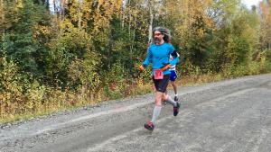
Andrea and I are running the Equinox Marathon relay this Saturday with Norwegian dog musher Halvor Hoveid. He’s running the first leg, I’m running the second, and Andrea finishes the race. I ran the second leg as a training run a couple weeks ago and feel good about my physical conditioning, but the weather is always a concern this late in the fall, especially up on top of Ester Dome, where it can be dramatically different than the valley floor where the race starts and ends.
Andrea ran the full marathon in 2009—2012 and the relay in 2008 and 2013—2015. I ran the full marathon in 2013. There was snow on the trail when I ran it, making the out and back section slippery and treacherous, and the cold temperatures at the start meant my feet were frozen until I got off of the single-track, nine or ten miles into the course. In other years, rain turned the powerline section to sloppy mud, or cold temperatures and freezing rain up on the Dome made it unpleasant for runners and supporters.
In this post we will examine the available weather data, looking at the range of conditions we could experience this weekend. The current forecast from the National Weather Service is calling for mostly cloudy skies with highs in the 50s. Low temperatures the night before are predicted to be in the 40s, with rain in the forecast between now and then.
Methods
There is no long term climate data for Ester Dome, but there are several valley-level stations with data going back to the start of the race in 1963. The best data comes from the Fairbanks Airport station and includes daily temperature, precipitation, and snowfall for all years, and wind speed and direction since 1984. I also looked at the data from the College Observatory station (FAOA2) behind the GI on campus and the University Experimental Farm, also on campus, but neither of these stations have a complete record. The daily data is part of the Global Historical Climatology Network - Daily dataset.
I also have hourly data from 2008—2013 for both the Fairbanks Airport and a station located on Ester Dome that is no longer operational. We’ll use this to get a sense of what the possible temperatures on Ester Dome might have been based on the Fairbanks Airport data. Hourly data comes from the Meterological Assimilation Data Ingest System (MADIS).
The R code used for this post appears at the bottom, and all the data used is available from here.
Results
Ester Dome temperatures
Since there isn’t a long-running weather station on Ester Dome (at least not one that’s publicly available), we’ll use the September data from an hourly Ester Dome station that was operational until 2014. If we join the Fairbanks Airport station data with this data wherever the observations are within 30 minutes of each other, we can see the relationship between Ester Dome temperature and temperature at the Fairbanks Airport.
Here’s what that relationship looks like, including a linear regression line between the two. The shaded area in the lower left corner shows the region where the temperatures on Ester Dome are below freezing.

And the regression:
##
## Call:
## lm(formula = ester_dome_temp_f ~ pafa_temp_f, data = pafa_fbsa)
##
## Residuals:
##    Min     1Q Median     3Q    Max
## -9.649 -3.618 -1.224  2.486 22.138
##
## Coefficients:
##             Estimate Std. Error t value Pr(>|t|)
## (Intercept) -2.69737    0.77993  -3.458 0.000572 ***
## pafa_temp_f  0.94268    0.01696  55.567  < 2e-16 ***
## ---
## Signif. codes:  0 '***' 0.001 '**' 0.01 '*' 0.05 '.' 0.1 ' ' 1
##
## Residual standard error: 5.048 on 803 degrees of freedom
## Multiple R-squared:  0.7936, Adjusted R-squared:  0.7934
## F-statistic:  3088 on 1 and 803 DF,  p-value: < 2.2e-16
The regression model is highly significant, as are both coefficients, and the relationship explains almost 80% of the variation in the data. According to the model, in the month of September, Ester Dome average temperature is almost three degrees colder than at the airport. And whenever temperature at the airport drops below 37 degrees, it’s probably below freezing on the Dome.
Race day weather
Temperatures at the airport on race day ranged from 19.9 °F in 1972 to 68 °F in 1969, and the range of average temperatures is 34.2 and 53 °F. Using our model of Ester Dome temperatures, we get an average range of 29.5 and 47 °F and an overall min / max of 16.1 / 61.4 °F. Generally speaking, in most years it will be below freezing on Ester Dome, but possibly before most of the runners get up there.
Precipitation (rain, sleet, or snow) has fallen on 15 out of 53 race days, or 28% of the time, and measurable snowfall has been recorded on four of those fifteen. The highest amount fell in 2014 with 0.36 inches of liquid precipitation (no snow was recorded and the temperatures were between 45 and 51 °F so it was almost certainly all rain, even on Ester Dome). More than a quarter of an inch of precipitation fell in three of the fifteen years (1990, 1992, and 2014), but most rainfall totals are much smaller.
Measurable snow fell at the airport in four years, or seven percent of the time: 4.1 inches in 1993, 2.1 inches in 1985, 1.2 inches in 1996 and 0.4 inches in 1992. But that’s at the airport station. Four of the 15 years where measurable precipitation fell at the airport, but no snow fell, had possible minimum temperatures on Ester Dome that were below freezing. It’s likely that some of the precipitation recorded at the airport in those years was coming down as snow up on Ester Dome. If so, that means snow may have fallen on eight race days, bringing the percentage up to fifteen percent.
Wind data from the airport has only been recorded since 1984, but from those years the average wind speed at the airport on race day is 4.9 miles per hour. Peak 2-minute winds during Equinox race day was 21 miles per hour in 2003. Unfortunately, no wind data is available for Ester Dome, but it’s likely to be higher than what is recorded at the airport. We do have wind speed data from the hourly Ester Dome station from 2008 through 2013, but the linear relationship between Ester Dome winds and winds at the Fairbanks airport only explain about a quarter of the variation in the data, and a look at the plot doesn’t give me much confidence in the relationship shown (see below).

Weather from the week prior
It’s also useful to look at the weather from the week before the race, since excessive pre-race rain or snow can make conditions on race day very different, even if the race day weather is pleasant. The year I ran the full marathon (2013), it had snowed the week before and much of the trail in the woods before the water stop near Henderson and all of the out and back were covered in snow.
The most dramatic example of this was 1992 where 23 inches of snow fell at the airport in the week prior to the race, with much higher totals up on the summit of Ester Dome. Measurable snow has been recorded at the airport in the week prior to six races, but all the weekly totals are under an inch except for the snow year of 1992.
Precipitation has fallen in 42 of 53 pre-race weeks (79% of the time). Three years have had more than an inch of precipitation prior to the race: 1.49 inches in 2015, 1.26 inches in 1992 (which fell as snow), and 1.05 inches in 2007. On average, just over two tenths of an inch of precipitation falls in the week before the race.
Summary
The following stacked plots shows the weather for all 53 runnings of the Equinox marathon. The top panel shows the range of temperatures on race day from the airport station (wide bars) and estimated on Ester Dome (thin lines below bars). The shaded area at the bottom shows where temperatures are below freezing. Dashed orange horizonal lines represent the average high and low temperature at the airport on race day; solid orange horizonal lines indicate estimated average high and low temperature on Ester Dome.
The middle panel shows race day liquid precipitation (rain, melted snow). Bars marked with an asterisk indicate years where snow was also recorded at the airport, but remember that four of the other years with liquid precipitation probably experienced snow on Ester Dome (1977, 1986, 1991, and 1994) because the temperatures were likely to be below freezing at elevation.
The bottom panel shows precipitation totals from the week prior to the race. Bars marked with an asterisk indicate weeks where snow was also recorded at the airport.

Here’s a table with most of the data from the analysis. Record values for each variable are in bold.
| Fairbanks Airport Station | Ester Dome (estimated) | ||||||||
|---|---|---|---|---|---|---|---|---|---|
| Race Day | Previous Week | Race Day | |||||||
| Date | min t | max t | wind | prcp | snow | prcp | snow | min t | max t |
| 1963‑09‑21 | 32.0 | 54.0 | 0.00 | 0.0 | 0.01 | 0.0 | 27.5 | 48.2 | |
| 1964‑09‑19 | 34.0 | 57.9 | 0.00 | 0.0 | 0.03 | 0.0 | 29.4 | 51.9 | |
| 1965‑09‑25 | 37.9 | 60.1 | 0.00 | 0.0 | 0.80 | 0.0 | 33.0 | 54.0 | |
| 1966‑09‑24 | 36.0 | 62.1 | 0.00 | 0.0 | 0.01 | 0.0 | 31.2 | 55.8 | |
| 1967‑09‑23 | 35.1 | 57.9 | 0.00 | 0.0 | 0.00 | 0.0 | 30.4 | 51.9 | |
| 1968‑09‑21 | 23.0 | 44.1 | 0.00 | 0.0 | 0.04 | 0.0 | 19.0 | 38.9 | |
| 1969‑09‑20 | 35.1 | 68.0 | 0.00 | 0.0 | 0.00 | 0.0 | 30.4 | 61.4 | |
| 1970‑09‑19 | 24.1 | 39.9 | 0.00 | 0.0 | 0.42 | 0.0 | 20.0 | 34.9 | |
| 1971‑09‑18 | 35.1 | 55.9 | 0.00 | 0.0 | 0.14 | 0.0 | 30.4 | 50.0 | |
| 1972‑09‑23 | 19.9 | 42.1 | 0.00 | 0.0 | 0.01 | 0.2 | 16.1 | 38.0 | |
| 1973‑09‑22 | 30.0 | 44.1 | 0.00 | 0.0 | 0.05 | 0.0 | 25.6 | 38.9 | |
| 1974‑09‑21 | 48.0 | 60.1 | 0.08 | 0.0 | 0.00 | 0.0 | 42.6 | 54.0 | |
| 1975‑09‑20 | 37.9 | 55.9 | 0.02 | 0.0 | 0.02 | 0.0 | 33.0 | 50.0 | |
| 1976‑09‑18 | 34.0 | 59.0 | 0.00 | 0.0 | 0.54 | 0.0 | 29.4 | 52.9 | |
| 1977‑09‑24 | 36.0 | 48.9 | 0.06 | 0.0 | 0.20 | 0.0 | 31.2 | 43.4 | |
| 1978‑09‑23 | 30.0 | 42.1 | 0.00 | 0.0 | 0.10 | 0.3 | 25.6 | 37.0 | |
| 1979‑09‑22 | 35.1 | 62.1 | 0.00 | 0.0 | 0.17 | 0.0 | 30.4 | 55.8 | |
| 1980‑09‑20 | 30.9 | 43.0 | 0.00 | 0.0 | 0.35 | 0.0 | 26.4 | 37.8 | |
| 1981‑09‑19 | 37.0 | 43.0 | 0.15 | 0.0 | 0.04 | 0.0 | 32.2 | 37.8 | |
| 1982‑09‑18 | 42.1 | 61.0 | 0.02 | 0.0 | 0.22 | 0.0 | 37.0 | 54.8 | |
| 1983‑09‑17 | 39.9 | 46.9 | 0.00 | 0.0 | 0.05 | 0.0 | 34.9 | 41.5 | |
| 1984‑09‑22 | 28.9 | 60.1 | 5.8 | 0.00 | 0.0 | 0.08 | 0.0 | 24.5 | 54.0 |
| 1985‑09‑21 | 30.9 | 42.1 | 6.5 | 0.14 | 2.1 | 0.57 | 0.0 | 26.4 | 37.0 |
| 1986‑09‑20 | 36.0 | 52.0 | 8.3 | 0.07 | 0.0 | 0.21 | 0.0 | 31.2 | 46.3 |
| 1987‑09‑19 | 37.9 | 61.0 | 6.3 | 0.00 | 0.0 | 0.00 | 0.0 | 33.0 | 54.8 |
| 1988‑09‑24 | 37.0 | 45.0 | 4.0 | 0.00 | 0.0 | 0.11 | 0.0 | 32.2 | 39.7 |
| 1989‑09‑23 | 36.0 | 61.0 | 8.5 | 0.00 | 0.0 | 0.07 | 0.5 | 31.2 | 54.8 |
| 1990‑09‑22 | 37.9 | 50.0 | 7.8 | 0.26 | 0.0 | 0.00 | 0.0 | 33.0 | 44.4 |
| 1991‑09‑21 | 36.0 | 57.0 | 4.5 | 0.04 | 0.0 | 0.03 | 0.0 | 31.2 | 51.0 |
| 1992‑09‑19 | 24.1 | 33.1 | 6.7 | 0.01 | 0.4 | 1.26 | 23.0 | 20.0 | 28.5 |
| 1993‑09‑18 | 28.0 | 37.0 | 4.9 | 0.29 | 4.1 | 0.37 | 0.3 | 23.7 | 32.2 |
| 1994‑09‑24 | 27.0 | 51.1 | 6.0 | 0.02 | 0.0 | 0.08 | 0.0 | 22.8 | 45.5 |
| 1995‑09‑23 | 43.0 | 66.9 | 4.0 | 0.00 | 0.0 | 0.00 | 0.0 | 37.8 | 60.4 |
| 1996‑09‑21 | 28.9 | 37.9 | 6.9 | 0.06 | 1.2 | 0.26 | 0.0 | 24.5 | 33.0 |
| 1997‑09‑20 | 27.0 | 55.0 | 3.8 | 0.00 | 0.0 | 0.03 | 0.0 | 22.8 | 49.2 |
| 1998‑09‑19 | 42.1 | 60.1 | 4.9 | 0.00 | 0.0 | 0.37 | 0.0 | 37.0 | 54.0 |
| 1999‑09‑18 | 39.0 | 64.9 | 3.8 | 0.00 | 0.0 | 0.26 | 0.0 | 34.1 | 58.5 |
| 2000‑09‑16 | 28.9 | 50.0 | 5.6 | 0.00 | 0.0 | 0.30 | 0.0 | 24.5 | 44.4 |
| 2001‑09‑22 | 33.1 | 57.0 | 1.6 | 0.00 | 0.0 | 0.00 | 0.0 | 28.5 | 51.0 |
| 2002‑09‑21 | 33.1 | 48.9 | 3.8 | 0.00 | 0.0 | 0.03 | 0.0 | 28.5 | 43.4 |
| 2003‑09‑20 | 26.1 | 46.0 | 9.6 | 0.00 | 0.0 | 0.00 | 0.0 | 21.9 | 40.7 |
| 2004‑09‑18 | 26.1 | 48.0 | 4.3 | 0.00 | 0.0 | 0.25 | 0.0 | 21.9 | 42.6 |
| 2005‑09‑17 | 37.0 | 63.0 | 0.9 | 0.00 | 0.0 | 0.09 | 0.0 | 32.2 | 56.7 |
| 2006‑09‑16 | 46.0 | 64.0 | 4.3 | 0.00 | 0.0 | 0.00 | 0.0 | 40.7 | 57.6 |
| 2007‑09‑22 | 25.0 | 45.0 | 4.7 | 0.00 | 0.0 | 1.05 | 0.0 | 20.9 | 39.7 |
| 2008‑09‑20 | 34.0 | 51.1 | 4.5 | 0.00 | 0.0 | 0.08 | 0.0 | 29.4 | 45.5 |
| 2009‑09‑19 | 39.0 | 50.0 | 5.8 | 0.00 | 0.0 | 0.25 | 0.0 | 34.1 | 44.4 |
| 2010‑09‑18 | 35.1 | 64.9 | 2.5 | 0.00 | 0.0 | 0.00 | 0.0 | 30.4 | 58.5 |
| 2011‑09‑17 | 39.9 | 57.9 | 1.3 | 0.00 | 0.0 | 0.44 | 0.0 | 34.9 | 51.9 |
| 2012‑09‑22 | 46.9 | 66.9 | 6.0 | 0.00 | 0.0 | 0.33 | 0.0 | 41.5 | 60.4 |
| 2013‑09‑21 | 24.3 | 44.1 | 5.1 | 0.00 | 0.0 | 0.13 | 0.6 | 20.2 | 38.9 |
| 2014‑09‑20 | 45.0 | 51.1 | 1.6 | 0.36 | 0.0 | 0.00 | 0.0 | 39.7 | 45.5 |
| 2015‑09‑19 | 37.9 | 44.1 | 2.9 | 0.01 | 0.0 | 1.49 | 0.0 | 33.0 | 38.9 |
Postscript
The weather for the 2016 race was just about perfect with temperatures ranging from 34 to 58 °F and no precipitation during the race. The airport did record 0.01 inches for the day, but this fell in the evening, after the race had finished.
Appendix: R code
 library(dplyr)
 library(readr)
 library(lubridate)
 library(ggplot2)
 library(scales)
 library(grid)
 library(gtable)

 race_dates <- read_fwf("equinox_marathon_dates.rst", skip=5, n_max=54,
                        fwf_positions(c(4, 6), c(9, 19), c("number", "race_date")))

 noaa <- src_postgres(host="localhost", dbname="noaa")
 # pivot <- tbl(noaa, build_sql("SELECT * FROM ghcnd_pivot
 #                               WHERE station_name = 'UNIVERSITY EXP STN'"))
 # pivot <- tbl(noaa, build_sql("SELECT * FROM ghcnd_pivot
 #                               WHERE station_name = 'COLLEGE OBSY'"))
 pivot <- tbl(noaa, build_sql("SELECT * FROM ghcnd_pivot
                               WHERE station_name = 'FAIRBANKS INTL AP'"))

 race_day_wx <- pivot %>%
     inner_join(race_dates, by=c("dte"="race_date"), copy=TRUE) %>%
     collect() %>%
     mutate(tmin_f=round((tmin_c*9/5.0)+32, 1), tmax_f=round((tmax_c*9/5.0)+32, 1),
            prcp_in=round(prcp_mm/25.4, 2),
            snow_in=round(snow_mm/25.4, 1), snwd_in=round(snow_mm/25.4, 1),
            awnd_mph=round(awnd_mps*2.2369, 1),
            wsf2_mph=round(wsf2_mps*2.2369), 1) %>%
     select(number, race_date, tmin_f, tmax_f, prcp_in, snow_in,
            snwd_in, awnd_mph, wsf2_mph)

 week_before_race_day_wx <- pivot %>%
     mutate(year=date_part("year", dte)) %>%
     inner_join(race_dates %>%
                    mutate(year=year(race_date)),
                copy=TRUE) %>%
     collect() %>%
     mutate(tmin_f=round((tmin_c*9/5.0)+32, 1), tmax_f=round((tmax_c*9/5.0)+32, 1),
            prcp_in=round(prcp_mm/25.4, 2),
            snow_in=round(snow_mm/25.4, 1), snwd_in=round(snow_mm/25.4, 1),
            awnd_mph=round(awnd_mps*2.2369, 1), wsf2_mph=round(wsf2_mps*2.2369, 1)) %>%
     select(number, year, race_date, dte, prcp_in, snow_in) %>%
     mutate(week_before=race_date-days(7)) %>%
     filter(dte<race_date, dte>=week_before) %>%
     group_by(number, year, race_date) %>%
     summarize(pweek_prcp_in=sum(prcp_in),
               pweek_snow_in=sum(snow_in))

 all_wx <- race_day_wx %>%
     inner_join(week_before_race_day_wx) %>%
     mutate(tavg_f=(tmin_f+tmax_f)/2.0,
            snow_label=ifelse(snow_in>0, '*', NA),
            pweek_snow_label=ifelse(pweek_snow_in>0, '*', NA)) %>%
     select(number, year, race_date, tmin_f, tmax_f, tavg_f,
            prcp_in, snow_in, snwd_in, awnd_mph, wsf2_mph,
            pweek_prcp_in, pweek_snow_in,
            snow_label, pweek_snow_label);

 write_csv(all_wx, "all_wx.csv")

 madis <- src_postgres(host="localhost", dbname="madis")

 pafa_fbsa <- tbl(madis,
                  build_sql("
   WITH pafa AS (
     SELECT dt_local, temp_f, wspd_mph
     FROM observations
     WHERE station_id = 'PAFA' AND date_part('month', dt_local) = 9),
   fbsa AS (
     SELECT dt_local, temp_f, wspd_mph
     FROM observations
     WHERE station_id = 'FBSA2' AND date_part('month', dt_local) = 9)
   SELECT pafa.dt_local, pafa.temp_f AS pafa_temp_f, pafa.wspd_mph as pafa_wspd_mph,
     fbsa.temp_f AS ester_dome_temp_f, fbsa.wspd_mph as ester_dome_wspd_mph
   FROM pafa
     INNER JOIN fbsa ON
       pafa.dt_local BETWEEN fbsa.dt_local - interval '15 minutes'
         AND fbsa.dt_local + interval '15 minutes'")) %>% collect()

 write_csv(pafa_fbsa, "pafa_fbsa.csv")

 ester_dome_temps <- lm(data=pafa_fbsa,
                        ester_dome_temp_f ~ pafa_temp_f)

 summary(ester_dome_temps)
 # Model and coefficients are significant, r2 = 0.794
 # intercept = -2.69737, slope = 0.94268

 all_wx_with_ed <- all_wx %>%
   mutate(ed_min_temp_f=round(ester_dome_temps$coefficients[1]+
                              tmin_f*ester_dome_temps$coefficients[2], 1),
          ed_max_temp_f=round(ester_dome_temps$coefficients[1]+
                              tmax_f*ester_dome_temps$coefficients[2], 1))

 make_gt <- function(outside, instruments, chamber, width, heights) {
     gt1 <- ggplot_gtable(ggplot_build(outside))
     gt2 <- ggplot_gtable(ggplot_build(instruments))
     gt3 <- ggplot_gtable(ggplot_build(chamber))
     max_width <- unit.pmax(gt1$widths[2:3], gt2$widths[2:3], gt3$widths[2:3])
     gt1$widths[2:3] <- max_width
     gt2$widths[2:3] <- max_width
     gt3$widths[2:3] <- max_width
     gt <- gtable(widths = unit(c(width), "in"), heights = unit(heights, "in"))
     gt <- gtable_add_grob(gt, gt1, 1, 1)
     gt <- gtable_add_grob(gt, gt2, 2, 1)
     gt <- gtable_add_grob(gt, gt3, 3, 1)

     gt
 }

temps <- ggplot(data=all_wx_with_ed, aes(x=year, ymin=tmin_f, ymax=tmax_f, y=tavg_f)) +
   # geom_abline(intercept=32, slope=0, color="blue", alpha=0.25) +
   geom_rect(data=all_wx_with_ed %>% head(n=1),
            aes(xmin=-Inf, xmax=Inf, ymin=-Inf, ymax=32),
            fill="darkcyan", alpha=0.25) +
   geom_abline(aes(slope=0,
                  intercept=mean(all_wx_with_ed$tmin_f)),
               color="darkorange", alpha=0.50, linetype=2) +
   geom_abline(aes(slope=0,
                  intercept=mean(all_wx_with_ed$tmax_f)),
               color="darkorange", alpha=0.50, linetype=2) +
   geom_abline(aes(slope=0,
                  intercept=mean(all_wx_with_ed$ed_min_temp_f)),
               color="darkorange", alpha=0.50, linetype=1) +
   geom_abline(aes(slope=0,
                  intercept=mean(all_wx_with_ed$ed_max_temp_f)),
               color="darkorange", alpha=0.50, linetype=1) +
   geom_linerange(aes(ymin=ed_min_temp_f, ymax=ed_max_temp_f)) +
   # geom_smooth(method="lm", se=FALSE) +
   geom_linerange(size=3, color="grey30") +
   scale_x_continuous(name="", limits=c(1963, 2015), breaks=seq(1963, 2015, 2)) +
   scale_y_continuous(name="Temperature (deg F)", breaks=pretty_breaks(n=10)) +
   theme_bw() +
   theme(plot.margin=unit(c(1, 1, 0, 0.5), 'lines')) +  # t, r, b, l
   theme(axis.text.x=element_blank(), axis.title.x=element_blank(),
         axis.ticks.x=element_blank(), panel.grid.minor.x=element_blank()) +
   ggtitle("Weather during and in the week prior to the Equinox Marathon
            Fairbanks Airport Station")

 prcp <- ggplot(data=all_wx, aes(x=year, y=prcp_in)) +
     geom_bar(stat="identity") +
     geom_text(aes(y=prcp_in+0.025, label=snow_label)) +
     scale_x_continuous(name="", limits=c(1963, 2015), breaks=seq(1963, 2015)) +
     scale_y_continuous(name="Precipitation (inches)", breaks=pretty_breaks(n=5)) +
     theme_bw() +
     theme(plot.margin=unit(c(0, 1, 0, 0.5), 'lines')) +  # t, r, b, l
     theme(axis.text.x=element_blank(), axis.title.x=element_blank(),
           axis.ticks.x=element_blank(), panel.grid.minor.x=element_blank())

 pweek_prcp <- ggplot(data=all_wx, aes(x=year, y=pweek_prcp_in)) +
     geom_bar(stat="identity") +
     geom_text(aes(y=pweek_prcp_in+0.1, label=pweek_snow_label)) +
     scale_x_continuous(name="", limits=c(1963, 2015), breaks=seq(1963, 2015)) +
     scale_y_continuous(name="Pre-week precip (inches)", breaks=pretty_breaks(n=5)) +
     theme_bw() +
     theme(plot.margin=unit(c(0, 1, 0.5, 0.5), 'lines'),
           axis.text.x=element_text(angle=45, hjust=1, vjust=1),
           panel.grid.minor.x=element_blank())

 rescale <- 0.75
 full_plot <- make_gt(temps, prcp, pweek_prcp,
                      16*rescale,
                      c(7.5*rescale, 2.5*rescale, 3.0*rescale))
 pdf("equinox_weather_grid.pdf", height=13*rescale, width=16*rescale)
 grid.newpage()
 grid.draw(full_plot)
 dev.off()

 fai_ed_temps <- ggplot(data=pafa_fbsa, aes(x=pafa_temp_f, y=ester_dome_temp_f)) +
   geom_rect(data=pafa_fbsa %>% head(n=1),
               aes(xmin=-Inf, ymin=-Inf, xmax=(32+2.69737)/0.94268, ymax=32),
               color="black", fill="darkcyan", alpha=0.25) +
   geom_point(position=position_jitter()) +
   geom_smooth(method="lm", se=FALSE) +
   scale_x_continuous(name="Fairbanks Airport Temperature (degrees F)") +
   scale_y_continuous(name="Ester Dome Temperature (degrees F)") +
   theme_bw() +
   ggtitle("Relationship between Fairbanks Airport and Ester Dome Temperatures
           September, 2008-2013")

 pdf("pafa_fbsa_sept_temps.pdf", height=10.5, width=10.5)
 print(fai_ed_temps)
 dev.off()

 fai_ed_wspds <- ggplot(data=pafa_fbsa, aes(x=pafa_wspd_mph, y=ester_dome_wspd_mph)) +
   geom_point(position=position_jitter()) +
   geom_smooth(method="lm", se=FALSE) +
   scale_x_continuous(name="Fairbanks Airport Wind Speed (MPH)") +
   scale_y_continuous(name="Ester Dome Wind (MPH)") +
   theme_bw() +
   ggtitle("Relationship between Fairbanks Airport and Ester Dome Wind Speeds
           September, 2008-2013")

 pdf("pafa_fbsa_sept_wspds.pdf", height=10.5, width=10.5)
 print(fai_ed_wspds)
 dev.off()
Buddy
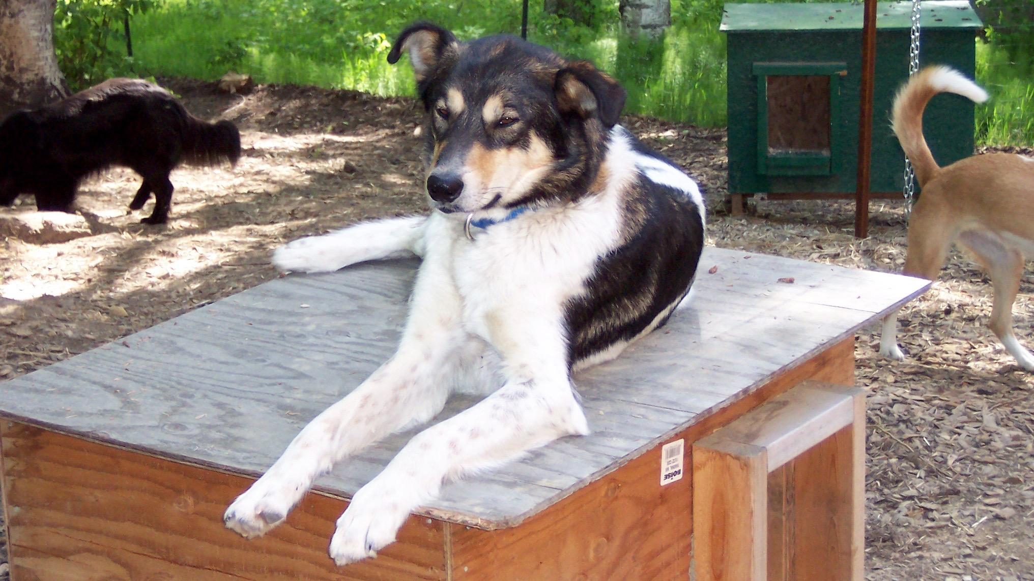
This morning I came down the stairs to a house without Buddy. He liked sleeping on the rug in front of the heater at the bottom of the stairs and he was always the first dog I saw in the morning.
Buddy came to us in August 2003 as a two year old and became Andrea’s mighty lead dog. He had the confidence to lead her teams even in single lead by himself, listened to whomever was driving, and tolerated all manner of misbehavior from whatever dog was next to him. He retired from racing after eleven years, but was still enjoying himself and pulling hard up to his last race.
Our friend, musher, and writer Carol Kaynor wrote this about him in 2012:
But it will be Buddy who will move me nearly to tears. He will drive for 6 full miles. On the very far side of 10 years old, with his eleventh birthday coming up in a month, he will bring us home to fourth place for the day and a respectable time for the distance. I’ll step off that sled as happy as if I’d won.
It wasn’t me pushing. I don’t get any credit for a run like that. It was Buddy pushing himself, like the champion he is.
Read the whole post here: Tribute to a champion.
After he retired, he enjoyed walking on the trails around our house, running around in the dog yard with the younger dogs, but most of all, relaxing in the house on the dog beds. He was a big, sweet, patient dog that took everything in stride and who wanted all the love and attention we could give him. The spot at the bottom of the stairs is empty now, and we will miss him.
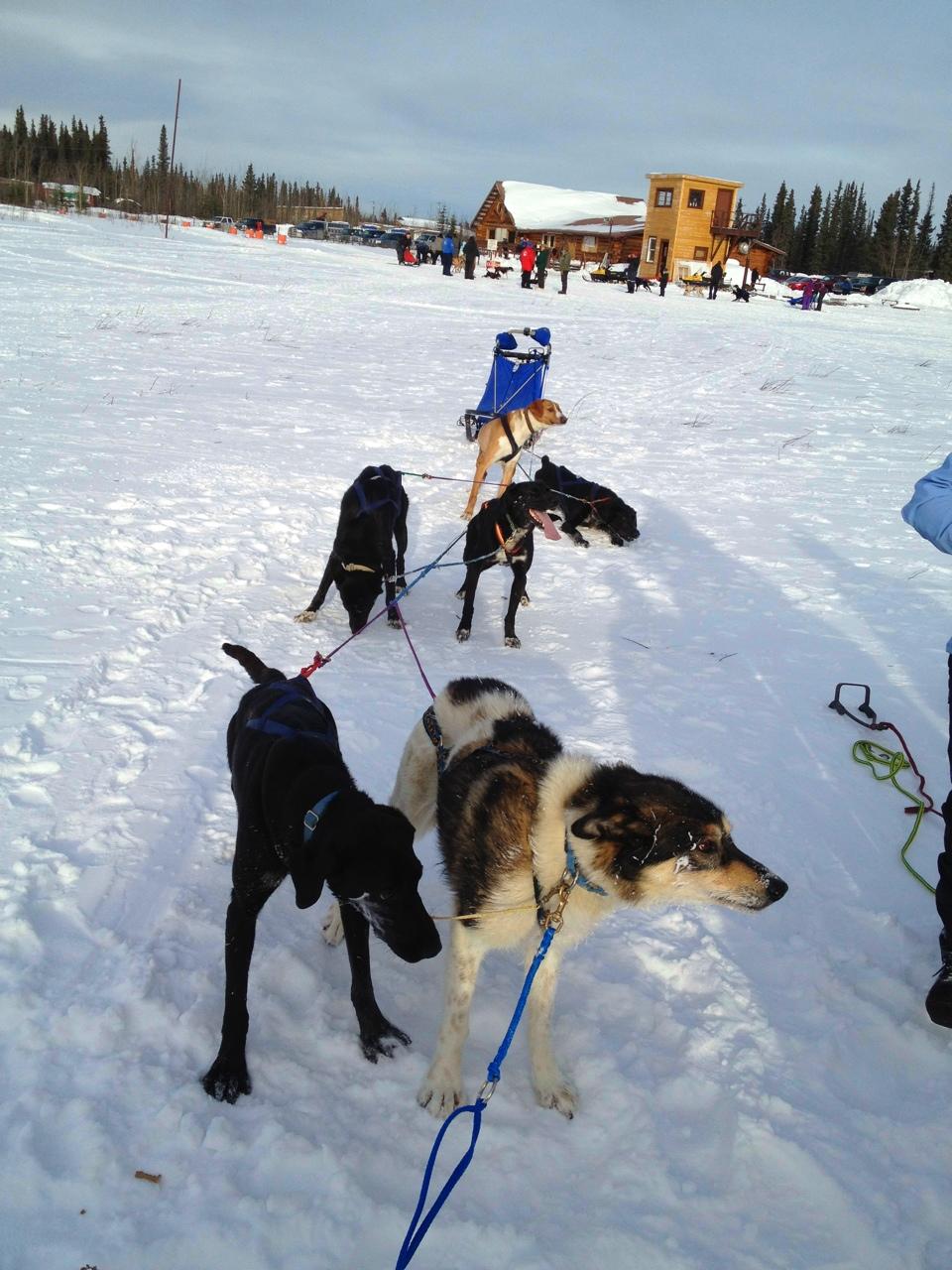
Buddy in lead in Tok, 2012
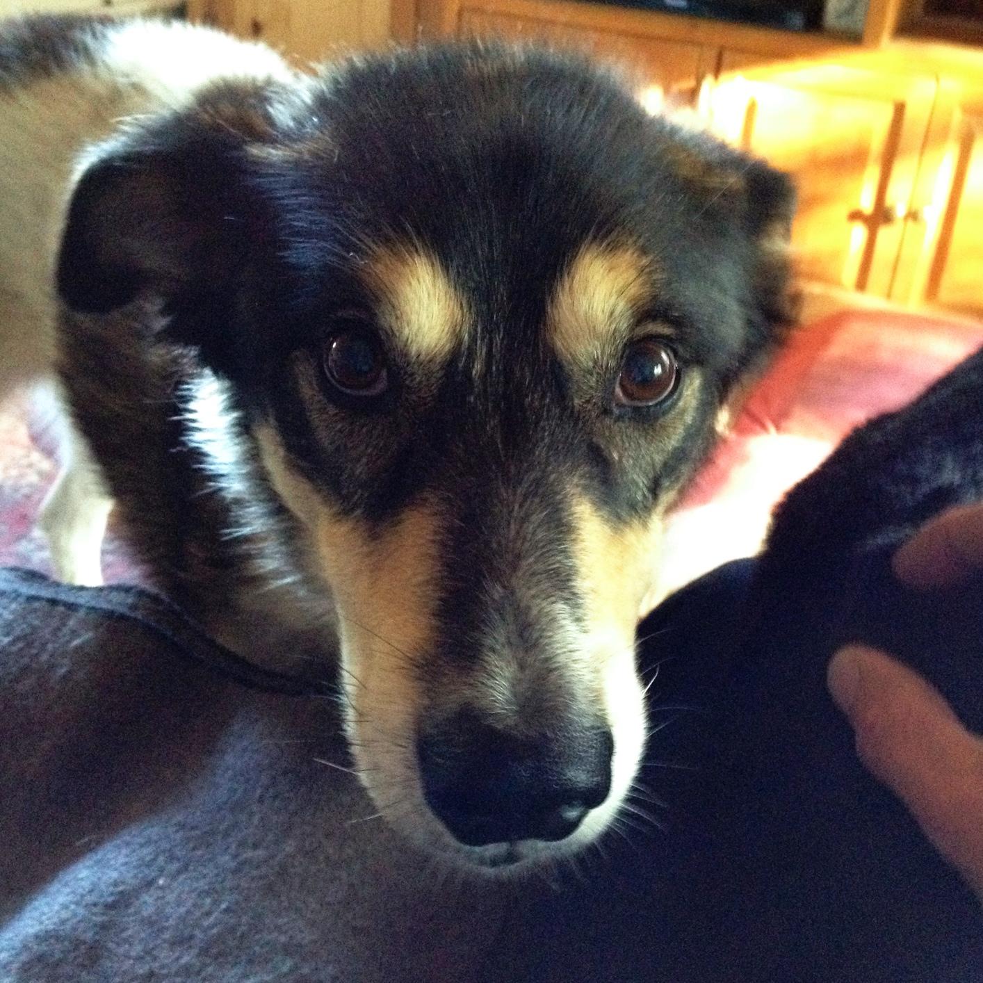
Mr. Buddy
This morning’s weather forecast:
SUNNY. HIGHS IN THE UPPER 70S TO LOWER 80S. LIGHT WINDS.
May 13th seems very early in the year to hit 80 degrees in Fairbanks, so I decided to check it out. What I’m doing here is selecting all the dates where the temperature is above 80°F, then ranking those dates by year and date, and extracting the “winner” for each year (where rank is 1).
WITH warm AS (
   SELECT extract(year from dte) AS year, dte,
      c_to_f(tmax_c) AS tmax_f
   FROM ghcnd_pivot
   WHERE station_name = 'FAIRBANKS INTL AP'
      AND c_to_f(tmax_c) >= 80.0),
ranked AS (
   SELECT year, dte, tmax_f,
      row_number() OVER (PARTITION BY year
                         ORDER BY dte) AS rank
   FROM warm)
SELECT dte,
   extract(doy from dte) AS doy,
   round(tmax_f, 1) as tmax_f
FROM ranked
WHERE rank = 1
ORDER BY doy;
And the results:
| Date | Day of year | High temperature (°F) |
|---|---|---|
| 1995-05-09 | 129 | 80.1 |
| 1975-05-11 | 131 | 80.1 |
| 1942-05-12 | 132 | 81.0 |
| 1915-05-14 | 134 | 80.1 |
| 1993-05-16 | 136 | 82.0 |
| 2002-05-20 | 140 | 80.1 |
| 2015-05-22 | 142 | 80.1 |
| 1963-05-22 | 142 | 84.0 |
| 1960-05-23 | 144 | 80.1 |
| 2009-05-24 | 144 | 80.1 |
| … | … | … |
If we hit 80°F today, it’ll be the fourth earliest day of year to hit that temperature since records started being kept in 1904.
Update: We didn’t reach 80°F on the 13th, but got to 82°F on May 14th, tied with that date in 1915 for the fourth earliest 80 degree temperature.