Today is the first time in a long time that I’ve been able to take both Nika and Piper out on the trails. For me, this is a turning point in a very long, stressful illness that Piper is still recovering from.
A couple months ago Piper got what we can only assume was an abscess inside her chest cavity. The result was that her chest filled with fluid and made breathing very difficult for her. The original diagnosis, made before she started having any real symptoms, was cancer, and we were preparing for the worst. Thankfully, Andrea didn’t give up on her, and several fantastic veterinarians in town didn’t either.
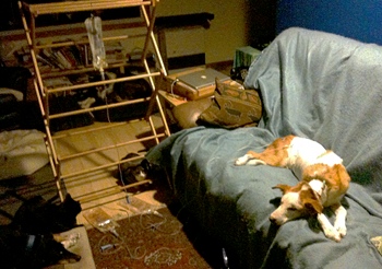
She spent some time in a hyperbaric chamber to get her oxygen levels up, and she had the fluids drained from her chest several times. Eventually, she had surgery to insert a pair of tubes into her chest, and we spent the next two weeks flushing her with fluids, every six hours. There’s a photo of the setup below. The procedure was to hook the saline bag to the input port on one side of her chest and put in 250 ml of fluid. Then we’d switch sides, and open the drain port on the side that had just been filled. Repeat until a liter has gone in and come back out again. The whole procedure took more than an hour, four times a day. At the same time, she was getting pain medication and antibiotics.
In the beginning, even after we had a good diagnosis, she was so sick that I don’t think anyone had much hope that she could be saved. She was too weak to stand without help and had a head tilt that seemed to indicate she’d gone septic. But as soon as we got some of the fluid out and the antibiotics started working on the infection inside her she improved dramatically.
Throughout all of it, Piper was fantastic. She went up on the couch to get treatment, went into her kennel at night, and handled all the trips to the vet without complaint or struggle.
She still has to take antibiotics for at least six months to make sure the infection really is gone, and it’s been a cold couple months because her chest was shaved prior to the surgery, but it’s all worth it. Seeing her running around on the trails today with Nika was a pleasure, and I think she enjoyed it too.
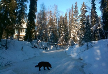
Nika, Goldstream Creek
The last couple days have seen a lot of overflow on Goldstream Creek, causing it to rise more than two feet. The water moved fast enough and it's been cold enough at night that it froze into a pretty good surface for ice skating. Many years ago we lived in a cabin at the edge of a pond near the railroad tracks and we bought ice skates so we skate on the pond. Turns out the number of days where the pond is frozen and not completely covered by snow is virtually zero, so we rarely got a chance to use them. But here, it seems that at least once or twice a year the overflow on the Creek or the DNR pond east of us will run over the snow and freeze into reasonably smooth ice.
I attempted to shoot a video while ice skating on the Creek today. It's not the greatest video, but it does give you some idea of what it looks like. After it freezes and before the overflow starts later in the winter, I spend a lot of time walking Nika and Piper down here. During breakup, the water rises to just below the bottom of the bridge, and then recedes to between four and five feet lower than where I'm skating by the middle of summer. The bridge I duck under is where I do my river stage measurements for the National Weather Service.
People always ask if we’re the coldest spot in town. I can’t really answer that, but I can find out if we’re the coldest reporting weather station in the region.
Once again, we’ll use PostgreSQL window functions to investigate. The following query finds the station in zone 222 (the National Weather Service region that includes Fairbanks) reporting the coldest temperature every hour during the winter, counts up all the stations that “won,” and then ranks them. The outermost query gets the total number of hourly winners and uses this to calculate the percentage of hours that each station was the coldest reporting station.
Check it out:
SELECT station, count,
    round(count / sum(count) OVER (
        ROWS BETWEEN UNBOUNDED PRECEDING AND UNBOUNDED FOLLOWING
    ) * 100, 1) AS percent
FROM (
    SELECT station, count(*) AS count
    FROM (
        SELECT station, dt_local, temp_f,
            rank() OVER (
                PARTITION BY dt_local ORDER BY temp_f
            )
        FROM (
            SELECT location || ' (' || station_id || ')' AS station,
                date_trunc('HOUR', dt_local) AS dt_local, temp_f
            FROM observations
                INNER JOIN stations USING (station_id)
            WHERE zone_id = 222
                AND dt_local between '2010-10-01' and '2011-03-31'
        ) AS foo
    ) AS bar WHERE bar.rank = 1 GROUP BY station ORDER BY count desc
) AS foobar;
And the results:
                station                 | count | percent
----------------------------------------+-------+---------
 Goldstream Creek (DW1454)              |  2156 |    51.0
 Chena Hot Springs (CNRA2)              |   484 |    11.5
 Eielson Air Force Base (PAEI)          |   463 |    11.0
 Parks Highway, MP 325.4 (NHPA2)        |   282 |     6.7
 Small Arms Range (SRGA2)               |   173 |     4.1
 Ballaine Road (AS115)                  |   153 |     3.6
 Fairbanks Airport (PAFA)               |   125 |     3.0
 Fort Wainwright (PAFB)                 |   107 |     2.5
 Ester Dome (FBSA2)                     |   103 |     2.4
 Eagle Ridge Road (C6333)               |    81 |     1.9
 Keystone Ridge (C5281)                 |    33 |     0.8
 Skyflight Ave (D6992)                  |    21 |     0.5
 14 Mile Chena Hot Springs Road (AP823) |    21 |     0.5
 College Observatory (FAOA2)            |    11 |     0.3
 Geophysical Institute (CRC)            |    10 |     0.2
 DGGS College Road (C6400)              |     1 |     0.0
Answer: Yep. We’re the coldest.
Update: Thinking about this a little bit more, the above analysis is biased against stations that don't report every hour. Another way to look at this is to calculate the hourly average temperature, subtract this from the data for each station during that hour, and then average those results for the whole winter. The query is made more complex because several stations report temperatures more than once an hour. If we simply averaged all these observations together with the stations that only reported once, these stations would bias the resulting hourly average. So we average each station's hourly data, then use that to calculate the zone average for the hour. Here's the query, and the results:
SELECT station,
    round(avg(diff), 1) AS avg_diff
FROM (
    SELECT station,
        dt_local,
        temp_f - avg(temp_f)
            OVER (
                PARTITION BY dt_local
                ROWS BETWEEN UNBOUNDED PRECEDING AND UNBOUNDED FOLLOWING
            ) AS diff
    FROM (
        SELECT location || ' (' || station_id || ')' AS station,
            date_trunc('HOUR', dt_local) AS dt_local,
            avg(temp_f) AS temp_f
        FROM observations
            INNER JOIN stations USING (station_id)
        WHERE zone_id = 222 AND
            dt_local between '2010-10-01' and '2011-03-31'
        GROUP BY station, date_trunc('HOUR', dt_local)
    ) AS foo
) AS bar
GROUP BY station
ORDER BY avg_diff;
                station                 | avg_diff
----------------------------------------+----------
 Goldstream Creek (DW1454)              |     -6.8
 Eielson Air Force Base (PAEI)          |     -3.8
 Fort Wainwright (PAFB)                 |     -3.1
 Fairbanks Airport (PAFA)               |     -2.9
 Small Arms Range (SRGA2)               |     -2.8
 Chena Hot Springs (CNRA2)              |     -2.3
 DGGS College Road (C6400)              |     -0.7
 Ballaine Road (AS115)                  |     -0.6
 College Observatory (FAOA2)            |      1.0
 North Bias Drive (RSQA2)               |      1.3
 14 Mile Chena Hot Springs Road (AP823) |      3.1
 Skyflight Ave (D6992)                  |      3.3
 Geophysical Institute (CRC)            |      3.5
 Eagle Ridge Road (C6333)               |      3.8
 Parks Highway, MP 325.4 (NHPA2)        |      4.5
 Keystone Ridge (C5281)                 |      5.1
 Ester Dome (FBSA2)                     |      5.1
 Birch Hill Recreation Area (BHS)       |      6.8
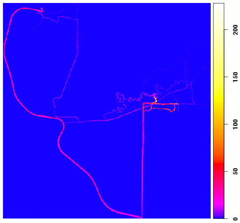
Location map
A couple years ago we got iPhones, and one of my favorite apps is the RunKeeper app, which tracks your outdoor activities using the phone’s built-in GPS. When I first started using it I compared the results of the tracks from the phone to a Garmin eTrex, and they were so close that I’ve given up carrying the Garmin. The fact that the phone is always with me, makes keeping track of all my walks with Nika, and trips to work on my bicycle or skis pretty easy. Just like having a camera with you all the time means you capture a lot more images of daily life, having a GPS with you means you have the opportunity to keep much better track of where you go.
RunKeeper records locations on your phone and transfers the data to the RunKeeper web site when you get home (or during your trip if you’ve got a good enough cell signal). Once on the web site, you can look at the tracks on a Google map, and RunKeeper generates all kinds of statistics on your travels. You can also download the data as GPX files, which is what I’m working with here.
The GPX files are processed by a Python script that inserts each point into a spatially-enabled PostgreSQL database (PostGIS), and ties it to a track.
Summary views allow me to generate statistics like this, a summary of all my travels in 2010:
| Type | Miles | Hours | Speed |
| Bicycling | 538.68 | 39.17 | 13.74 |
| Hiking | 211.81 | 92.84 | 2.29 |
| Skiing | 3.17 | 0.95 | 3.34 |
Another cool thing I can do is use R to generate a map showing where I’ve spent the most time. That’s what’s shown in the image on the right. If you’re familiar at all with the west side of the Goldstream Valley, you’ll be able to identify the roads, Creek, and trails I’ve been on in the last two years. The scale bar is the number of GPS coordinates fell within that grid, and you can get a sense of where I’ve travelled most. I’m just starting to learn what R can do with spatial data, so this is a pretty crude “analysis,” but here’s how I did it (in R):
library(RPostgreSQL)
library(spatstat)
drv <- dbDriver("PostgreSQL")
con <- dbConnect(drv, dbname="new_gps", host="nsyn")
points <- dbGetQuery(con,
    "SELECT type,
        ST_X(ST_Transform(the_geom, 32606)) AS x,
        ST_Y(ST_Transform(the_geom, 32606)) AS y
     FROM points
        INNER JOIN tracks USING (track_id)
        INNER JOIN types USING (type_id)
     WHERE ST_Y(the_geom) > 60 AND ST_X(the_geom) > -148;"
)
points_ppp <- ppp(points$x, points$y, c(min(points$x), max(points$x)), c(min(points$y), max(points$y)))
Lab.palette <- colorRampPalette(c("blue", "magenta", "red", "yellow", "white"), bias=2, space="Lab")
spatstat.options(npixel = c(500, 500))
map <- pixellate(points_ppp)
png("loc_map.png", width = 700, height = 600)
image(map, col = Lab.palette(256), main = "Gridded location counts")
dev.off()
Here’s a similar map showing just my walks with Nika and Piper:
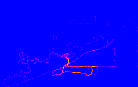
Walks with Nika and Piper
And here's something similar using ggplot2:
library(ggplot2)
m <- ggplot(data = points, aes(x = x, y = y)) + stat_density2d(geom = "tile", aes(fill = ..density..), contour = FALSE)
m + scale_fill_gradient2(low = "white", mid = "blue", high = "red", midpoint = 5e-07)
I trimmed off the legend and axis labels:
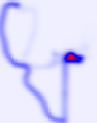
ggplot2, geom_density2d
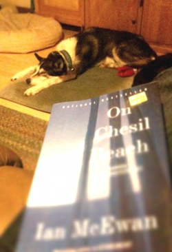
Deuce, On Chesil Beach
I’ve read a lot of Ian McEwan over the years, and it’s impressive how different his stories are, and how precise and well written they are. On Chesil Beach is a horror of a story where a single moment is fully visualized and expertly drawn, and when it, ahem, comes, you know that things will never be the same for the characters. I guess this is McEwan’s expertise: visualizing characters suddenly drawn into situations so far from their expectation that you never quite know how they will react.
In this case, one wonders if the outcome of the story would be different if the time or place were different? I should hope that a more modern sensibility, more open dialog about intimacy, perhaps even premarital sexual investigation, would prevent the sort of misunderstanding that’s at the center of this book.
Anyway, I enjoyed it, but I wasn’t as blown away as many of the reviewers were. I do like, oddly enough, what People magazine wrote about the book:
No one can unpack a single frozen moment better than McEwan.
Very true.

